Operationalize Variables

Published

March 31, 2026

Getting Started

# load custom functions
source("src/utils/custom_functions.r")

# clear the global environment and set dependencies
.clear_global_environment()
.load_quarto_dependencies()

# load and activate packages
library(tidyverse)
library(slider)
library(dplyr)
library(tidyr)
library(stringr)
library(tibble)
library(purrr)

Functions

`categorize_ethnicity()`

Classify scholars into migrant-origin groups based on their country of origin code.

Arguments

data

Named list containing a demographics element with at least a country_id column.

Method

The function defines a set of minority country codes corresponding to the four largest migrant groups in the Netherlands (MA, TR, BQ, CW, SX, AW, SR) and adds a migrant column. Scholars from the Netherlands are coded "NL", scholars from minority-coded countries are coded "M4", scholars with a missing country code receive NA, and all others are coded "other". The new column is relocated to follow country_id.

categorize_ethnicity = function(data){
  minority_codes =  c('MA', 'TR', 'BQ', 'CW', 'SX', 'AW', 'SR')
  country_codes = c('US', 'DE', 'BE')

  data[['demographics']] = data[['demographics']] |>
    mutate(migrant = case_when(
      country_id == 'NL' ~ 'NL',
      # country_id %in% country_codes ~ 'B3', # Big 3 origins
      country_id %in% minority_codes ~ 'M4', # 4 Biggest Migrant groups NL
      is.na(country_id) ~ NA_character_,
      .default = "other"
    )) |>
    relocate(migrant, .after = 'country_id')

  return(data)
}

`clean_affilliations()`

Standardize university affiliation strings, extract the first valid affiliation per year, and count the number of affiliations per year.

Arguments

data

Named list containing a demographics element with university_* columns (one per measurement year).

Method

The function first normalizes raw affiliation strings across all university_* columns by replacing . with /, mapping LEIDEN to UL, RUG to UVG, and UCU to UU. It then splits each normalized string on / and extracts the first token that appears in a predefined list of valid university codes, storing the result in new university_*_first columns. Finally, it counts the number of non-missing affiliation tokens per year and stores this in university_*_k columns.

clean_affilliations = function(data){
  valid_universities = c(
    'uu', 'uva', 'rug', 'ru', 'ucu', 'leiden', 'eur',
    'uvt', 'uvg', 'vu', 'wur', 'ul'
  )

  data[['demographics']] = data[['demographics']] |>
    mutate(
      across(
        starts_with('university'),
        # clean and split university strings
        ~ .x |> str_replace('\\.', '/') |>
          str_replace(regex('LEIDEN', ignore_case = TRUE), 'UL')  |>
          str_replace('RUG', 'UVG') |>
          str_replace('UCU', 'UU')
      ),
      # get the first valid affiliation per author year
      across(
        starts_with('university'),
        # clean and split university strings
        ~ .x |> str_replace('\\.', '/') |>
          str_to_lower() |>
          str_split(pattern = '/') |>
          # select the first of valid universities
          sapply(\(chunks){
            chunks[chunks %in% valid_universities][1]
          }),
        .names = "{.col}_first"
      ),
      # calculate the number of affiliations
      across(
        starts_with('university') & !ends_with('first'),
        ~ .x |> str_replace('\\.', '/') |>
          str_to_lower() |>
          str_split(pattern = '/') |>
          sapply(\(chunks){
            length(chunks[!is.na(chunks)])
          }),
        .names = "{.col}_k"
      )
    )

  return(data)
}

`set_time_matrix()`

Build a symmetric 8×8 travel-time distance matrix between Dutch universities.

Arguments

None.

Method

The function defines the upper triangle of a travel-time matrix as a named numeric vector and constructs an 8×8 matrix with row and column labels UVG, VU, UVA, UL, EUR, UVT, UU, and RU. The lower triangle is filled by mirroring the upper triangle, producing a symmetric matrix which is returned.

set_time_matrix = function(){
  time_distance = c(
    UVG = c(0,    NA,   NA,    NA,    NA,    NA,    NA,    NA),
    VU  = c(2.52, 0,    NA,    NA,    NA,    NA,    NA,    NA),
    UVA = c(2.58, 0.52, 0,     NA,    NA,    NA,    NA,    NA),
    UL  = c(3.12, 0.91, 1.04,  0,     NA,    NA,    NA,    NA),
    EUR = c(3.17, 1.32, 1.38,  1.18,  0,     NA,    NA,    NA),
    EVT = c(3.30, 1.70, 1.57,  1.67,  1.35,  0,     NA,    NA),
    UU  = c(2.47, 0.98, 0.88,  1.40,  1.33,  1.36,  0,     NA),
    RU  = c(2.83, 1.90, 1.68,  2.23,  2.33,  1.30,  1.53,  0)
  )
  labs = c('UVG', 'VU', 'UVA', 'UL', 'EUR', 'UVT', 'UU', 'RU')

  # convert to symmetrical matrix
  T = matrix(time_distance,
    ncol = 8, nrow = 8, dimnames = list(labs, labs)
  )
  T[lower.tri(T)] = T[upper.tri(T)]
  return(T)
}

`create_affiliations_long()`

Reshape demographics to a long (uid × year × affiliation) table.

Arguments

demographics

A tibble with a uid column and one or more university_*_first columns (one per measurement year).

affix

Character string suffix used to select the relevant affiliation columns. Defaults to "first".

year_regex

Regular expression used to extract the two-digit year from column names. Defaults to "\\d{2}".

Method

The function selects uid and all columns ending in affix, pivots them to long format, extracts the two-digit year from the column name using year_regex and prepends "20" to produce a four-digit year string, retains uid, year, and value, and uppercases the affiliation codes.

create_affiliations_long <- function(demographics,
                                     affix = "first",
                                     year_regex = "\\d{2}") {
  demographics %>%
    select(uid, ends_with(affix)) %>%
    pivot_longer(
      cols = ends_with(affix),
      names_to = "name",
      values_to = "value"
    ) %>%
    mutate(year = paste0("20", str_extract(name, regex(year_regex)))) %>%
    select(uid, year, value) %>%
    mutate(value = toupper(value))
}

`create_time_lookup()`

Convert the travel-time matrix to a long-format lookup table for use in joins.

Arguments

T

A square numeric matrix of travel-time distances between universities, as returned by set_time_matrix().

Method

The function coerces the matrix to a long-format data frame via as.table(), converts it to a tibble, and renames the columns to value_i, value_j, and distance to align with the naming conventions used in dyad join operations.

create_time_lookup <- function(T) {
  as.data.frame(as.table(T)) %>%
    as_tibble() %>%
    rename(value_i = Var1, value_j = Var2, distance = Freq)
}

`create_pairs_with_distance()`

Build a dyadic table of all scholar pairs per year, enriched with institutional travel-time distances.

Arguments

affiliations

A long (uid × year × affiliation) tibble as returned by create_affiliations_long().

T_long

A long-format travel-time lookup table as returned by create_time_lookup().

drop_self

Logical. If TRUE, self-pairs (uid_i == uid_j) are removed. Defaults to FALSE.

Method

The function creates a distinct uid–year–affiliation key table and crosses all uid pairs within each year using tidyr::crossing(). If drop_self is TRUE, self-pairs are removed. It then left-joins affiliation codes for both the focal scholar and partner, drops rows where either affiliation is missing, and joins on T_long to attach distance, dropping pairs for which no travel-time is available.

create_pairs_with_distance <- function(affiliations, T_long, drop_self = FALSE) {
  aff_key <- affiliations %>% distinct(year, uid, value)

  pairs <- aff_key %>%
    group_by(year) %>%
    summarise(pairs = list(tidyr::crossing(uid_i = uid, uid_j = uid)), .groups = "drop") %>%
    unnest(pairs)

  if (drop_self) {
    pairs <- pairs %>% filter(uid_i != uid_j)
  }

  pairs %>%
    left_join(aff_key, by = c("year", "uid_i" = "uid")) %>%
    rename(value_i = value) %>%
    left_join(aff_key, by = c("year", "uid_j" = "uid")) %>%
    rename(value_j = value) %>%
    drop_na(value_i, value_j) %>%
    left_join(T_long, by = c("value_i", "value_j")) %>%
    drop_na(distance)
}

`make_year_matrix()`

Populate a full uid × uid distance matrix for a single year from a dyad table.

Arguments

df_year

A tibble with uid_i, uid_j, and distance columns for a single year, as produced by splitting the output of create_pairs_with_distance().

all_uids

Character vector defining the complete set of row and column names for the output matrix.

Method

The function initializes an NA matrix of dimension length(all_uids) × length(all_uids) with row and column names set to all_uids. It uses match() to resolve each dyad to row and column indices, discards pairs whose UIDs are not found in all_uids, and fills the corresponding cells with their distance values. The populated matrix is returned.

make_year_matrix <- function(df_year, all_uids) {
  M <- matrix(
    NA_real_,
    nrow = length(all_uids),
    ncol = length(all_uids),
    dimnames = list(all_uids, all_uids)
  )

  ii <- match(df_year$uid_i, all_uids)
  jj <- match(df_year$uid_j, all_uids)
  keep <- !is.na(ii) & !is.na(jj)

  M[cbind(ii[keep], jj[keep])] <- df_year$distance[keep]
  M
}

`create_distance_matrices()`

Produce a named list of uid × uid travel-time distance matrices, one per year.

Arguments

pairs_by_year

A dyadic tibble with year, uid_i, uid_j, and distance columns, as returned by create_pairs_with_distance().

all_uids

Character vector defining the shared set of row and column names for all yearly matrices.

Method

The function selects the four relevant columns, splits the tibble by year using group_split(), names each list element with its year string, and maps make_year_matrix() over each split to produce a consistently-dimensioned named list of distance matrices.

create_distance_matrices <- function(pairs_by_year, all_uids) {
  pairs_by_year %>%
    select(year, uid_i, uid_j, distance) %>%
    group_by(year) %>%
    group_split() %>%
    set_names(map_chr(., ~ unique(.x$year))) %>%
    map(~ make_year_matrix(.x, all_uids))
}

`add_distances()`

Orchestrate the institutional travel-time distance pipeline and attach the resulting per-year matrices to data.

Arguments

data

Named list containing a demographics element with processed university_*_first affiliation columns.

topics

Named list containing a dissim sub-list whose field element provides the reference UID ordering used to dimension the output matrices.

Method

The function calls create_affiliations_long() to reshape affiliations to long format, set_time_matrix() and create_time_lookup() to build the travel-time lookup, and create_pairs_with_distance() to compute all pairwise institutional distances per year. It extracts the reference UID set from topics[["dissim"]][["field"]][["2022"]] and passes it to create_distance_matrices() to produce consistently-dimensioned per-year matrices. The resulting list is stored in data[['distances']] and the updated list is returned.

add_distances <- function(data, topics){
  # affiliations
  affiliations <- create_affiliations_long(data[["demographics"]])

  # time lookup
  T = set_time_matrix()
  T_long <- create_time_lookup(T)

  # dyads + distance
  pairs_by_year <- create_pairs_with_distance(affiliations, T_long)

  # global uid set / ordering
  all_uids <- colnames(topics[["dissim"]][["field"]][["2022"]])

  # matrices per year
  data[['distances']] <- create_distance_matrices(pairs_by_year, all_uids)

  return(data)
}

Application

data = freadRDS2('scholars', location = "./data/clean/")
topics = freadRDS2('topics', location = './data/clean/')

data = data |>
  categorize_ethnicity() |>
  clean_affilliations() |>
  add_distances(topics)

fsaveRDS(data, 'data', location = "./data/analysis/")

[1] "SAVING: ./data/analysis/20260331data.Rds"

fsaveRDS(topics, 'topics', location = "./data/analysis/")

[1] "SAVING: ./data/analysis/20260331topics.Rds"

Migrate these plots to another document

top_n <- 25

data[["demographics"]] |>
  count(country_id, migrant, name = "n") |>
  arrange(n) |>
  tail(25) |>
  mutate(country_id = factor(country_id, levels = unique(country_id))) |>
  ggplot(aes(x = country_id, y = n, fill = migrant)) +
  geom_col() +
  coord_flip() +
  labs(x = NULL, y = "Count", fill = "Migrant", title = "Counts by country_id, split by migrant") +
  theme_minimal()

data[['demographics']] |>
  filter(!is.na(career_start)) |>
  ggplot(aes(x = career_start)) +
  geom_density() +
  labs(x = "Career start (year)", y = "Density", title = "Kernel density of career start") +
  theme_minimal()

data[['demographics']] |>
  filter(!is.na(h_index_22)) |>
  ggplot(aes(x = h_index_22)) +
  geom_density() +
  labs(x = "h_index", y = "Density", title = "Kernel density of h-index in 2022") +
  theme_minimal()

data[['demographics']] |>
  filter(!is.na(i10_index_21)) |>
  ggplot(aes(x = i10_index_21)) +
  geom_density() +
  labs(x = "i10_index", y = "Density", title = "Kernel density of i10-index in 2022") +
  theme_minimal()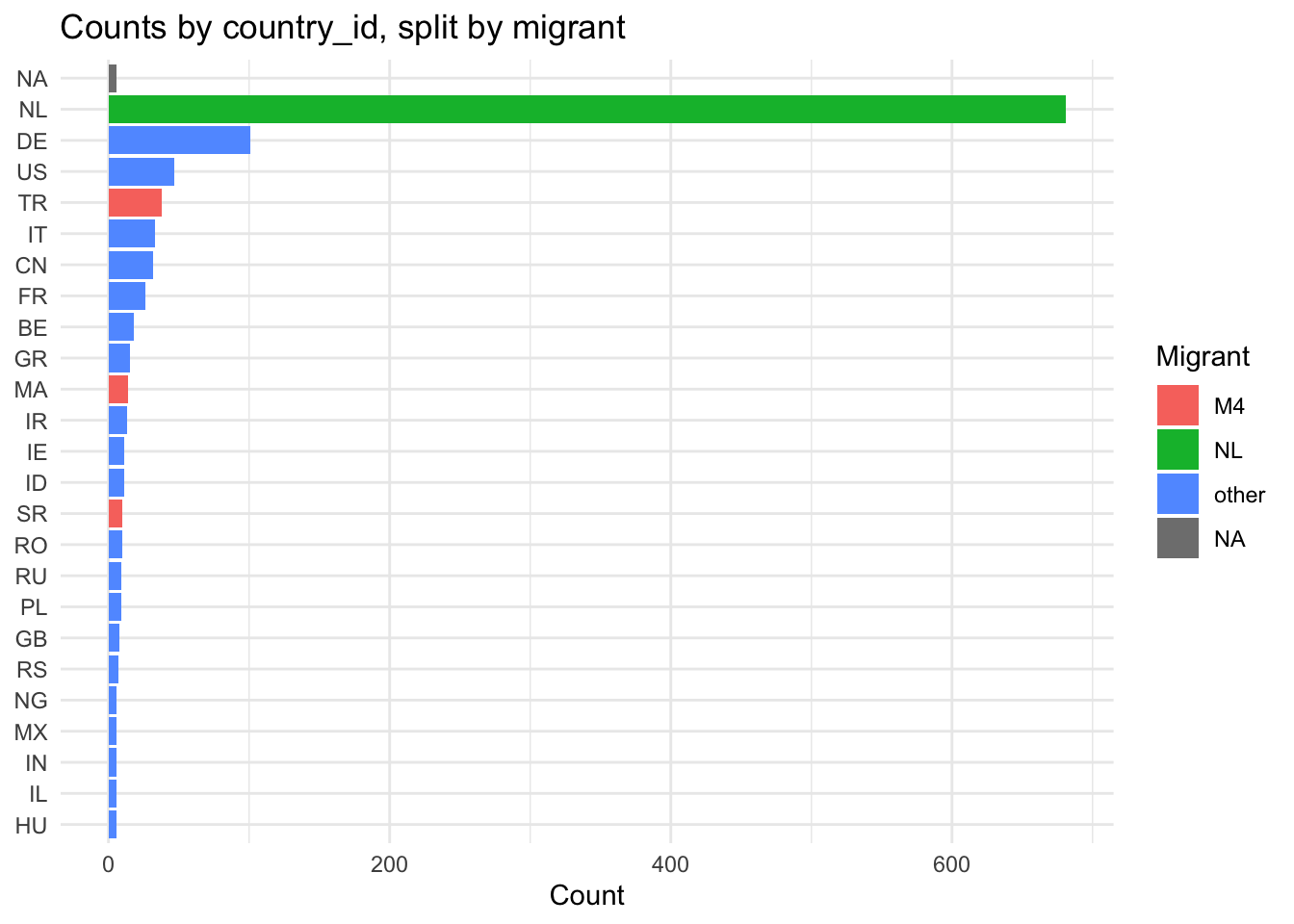

data[["demographics"]] |>
  group_by(position_22) |>
  summarise(has_valid_works = mean(!is.na(career_start)), .groups = "drop") |>
  arrange(desc(has_valid_works)) |>
  mutate(position_22 = factor(position_22, levels = position_22)) |>
  ggplot(aes(x = position_22, y = has_valid_works)) +
  geom_col() +
  coord_flip() +
  scale_y_continuous(limits = c(0, 1)) +
  labs(
    x = NULL,
    y = "Share with valid works",
    title = "Valid works by position (2025)"
  ) +
  theme_minimal()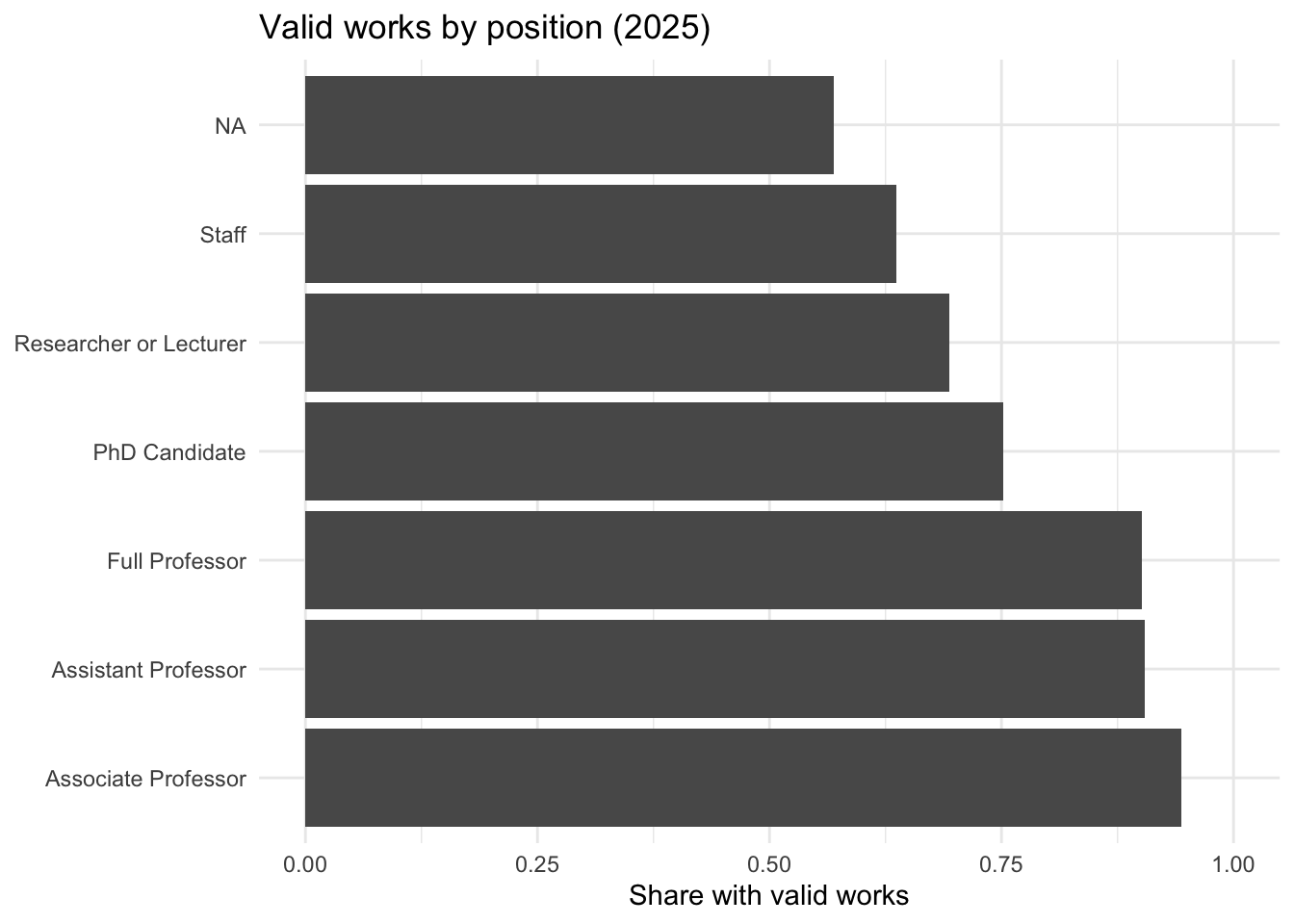

years <- c("2022", "2024", "2025")

dens_df <- map_dfr(years, function(y) {
  m <- topics[["dissim"]][["subfield"]][[y]]
  tibble(
    year = y,
    dissim = m[upper.tri(m)]
  )
}) |>
  filter(!is.na(dissim))

ggplot(dens_df, aes(x = dissim)) +
  geom_density() +
  facet_wrap(~ year, nrow = 1, scales = "free_y") +
  theme_minimal() +
  labs(x = "Dissimilarity (upper triangle)", y = "Density")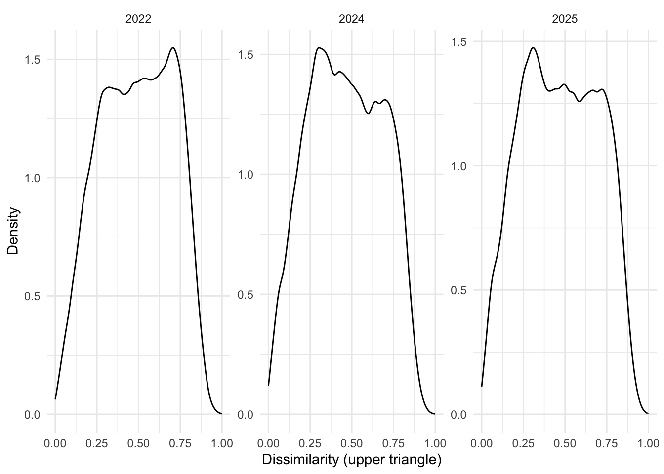

years <- c("2022", "2024", "2025")

dens_df <- map_dfr(years, function(y) {
  m <- topics[["dissim"]][["field"]][[y]]
  tibble(
    year = y,
    dissim = m[upper.tri(m)]
  )
}) |>
  filter(!is.na(dissim))

ggplot(dens_df, aes(x = dissim)) +
  geom_density() +
  facet_wrap(~ year, nrow = 1, scales = "free_y") +
  theme_minimal() +
  labs(x = "Dissimilarity (upper triangle)", y = "Density")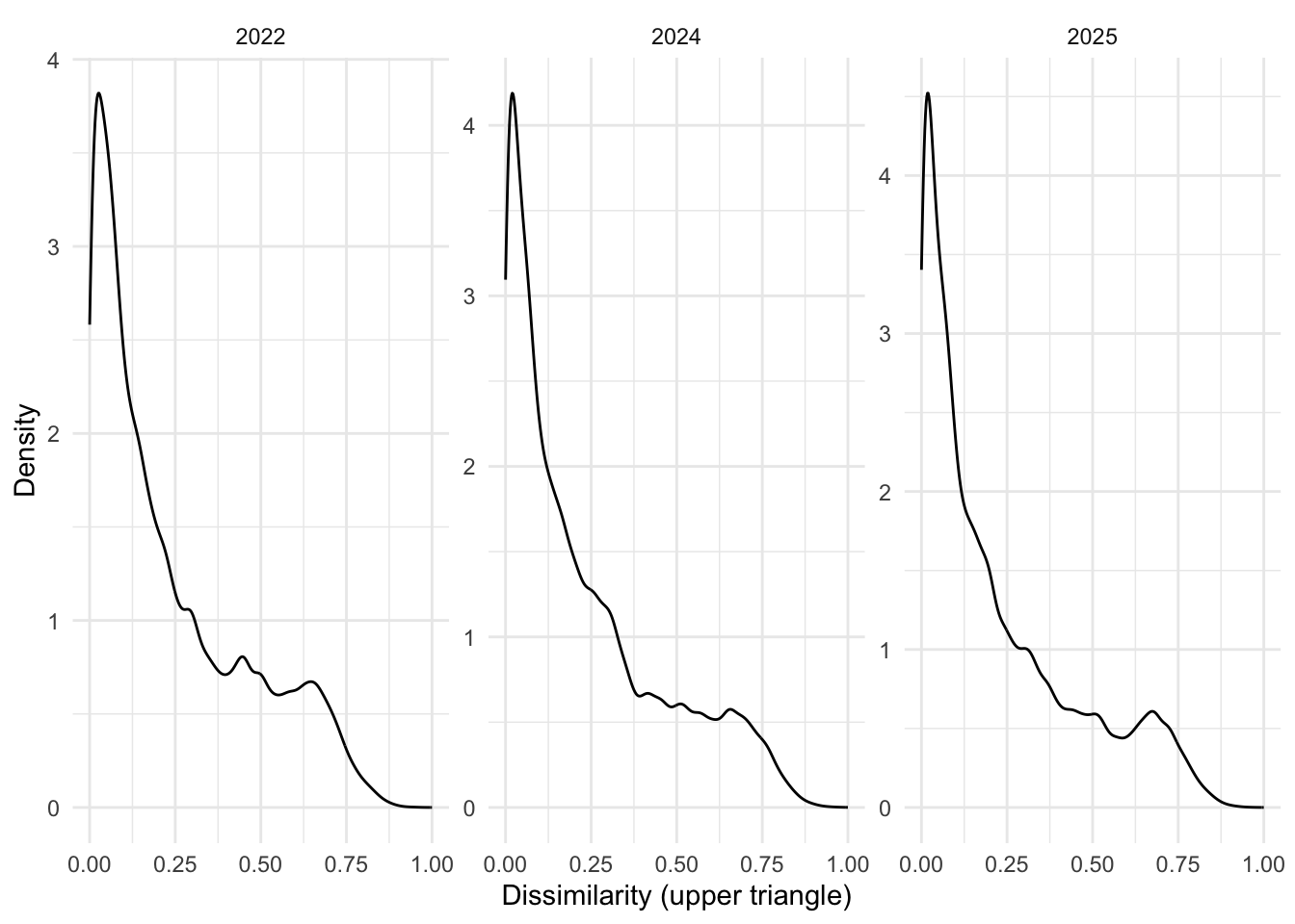

years <- c("2022", "2024", "2025")

dens_df <- map_dfr(years, function(y) {
  m <- topics[["dissim"]][["subfield"]][[y]]
  tibble(
    year = y,
    dissim = m[upper.tri(m)]
  )
}) |>
  filter(!is.na(dissim))

ggplot(dens_df, aes(x = dissim)) +
  geom_density() +
  facet_wrap(~ year, nrow = 1, scales = "free_y") +
  theme_minimal() +
  labs(x = "Dissimilarity (upper triangle)", y = "Density")

plot_df <- data[["demographics"]] |>
  select(uid, gender, university_22_first, university_24_first, university_25_first) |>
  pivot_longer(
    cols = starts_with("university_"),
    names_to = "year",
    values_to = "university"
  ) |>
  mutate(
    year = case_when(
      year == "university_22_first" ~ "2022",
      year == "university_24_first" ~ "2024",
      year == "university_25_first" ~ "2025",
      TRUE ~ year
    )
  ) |>
  filter(!is.na(university), university != "", !is.na(gender), gender != "") |>
  count(year, university, gender, name = "n") |>
  group_by(year, university) |>
  mutate(prop = n / sum(n)) |>
  ungroup()

ggplot(plot_df, aes(x = university, y = prop, fill = gender)) +
  geom_col() +
  facet_wrap(~ year, scales = "free_x") +
  scale_y_continuous(labels = scales::percent_format(accuracy = 1)) +
  theme_minimal() +
  theme(axis.text.x = element_text(angle = 45, hjust = 1)) +
  labs(x = NULL, y = "Gender composition", fill = "Gender")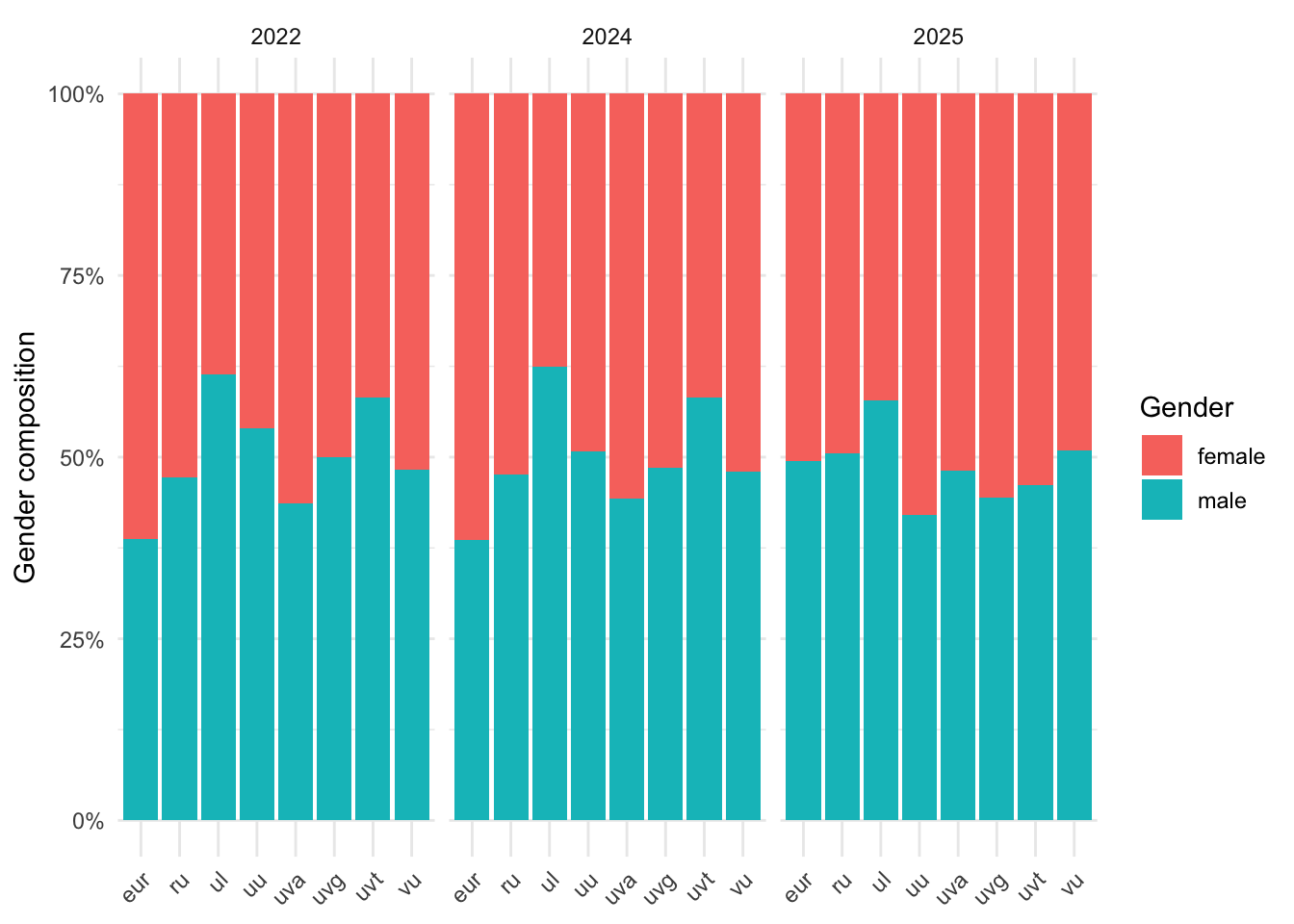

plot_df <- data[["demographics"]] |>
  select(university_22_first, university_24_first, university_25_first) |>
  pivot_longer(
    cols = everything(),
    names_to = "panel",
    values_to = "university"
  ) |>
  filter(!is.na(university), university != "") |>
  count(panel, university, name = "n")

ggplot(plot_df, aes(x = university, y = n)) +
  geom_col() +
  facet_wrap(~ panel, scales = "free_x") +
  theme_minimal() +
  theme(
    axis.text.x = element_text(angle = 45, hjust = 1),
    panel.spacing = unit(1, "lines")
  ) +
  labs(x = NULL, y = "Count")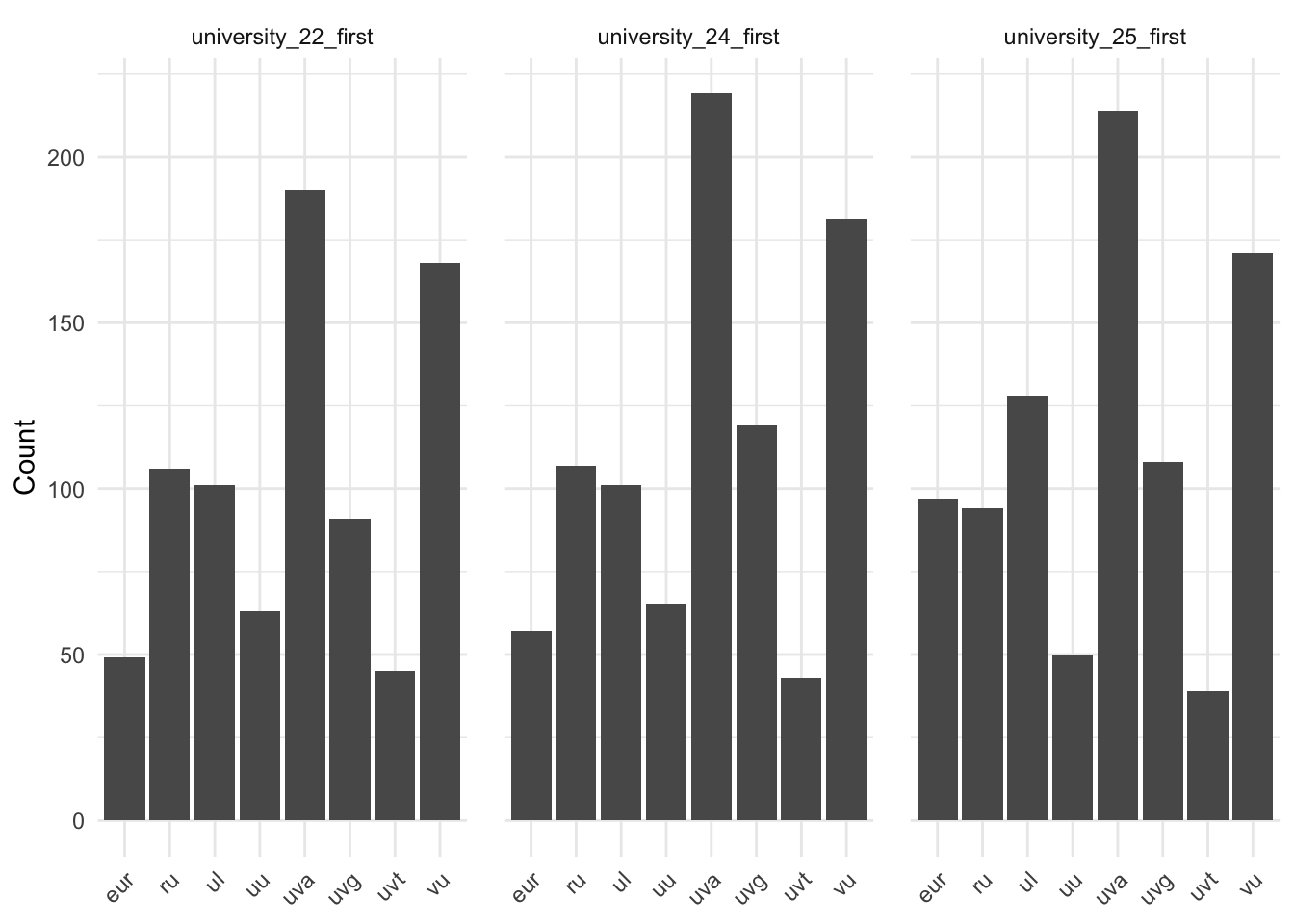

temp =  data[['demographics']] |>
  mutate(
    across(
      starts_with('university'),
      # clean and split university strings
      ~ .x |> str_replace('\\.', '/') |>
        str_replace(regex('LEIDEN', ignore_case = TRUE), 'UL')  |>
        str_replace('RUG', 'UVG') |>
        str_replace('UCU', 'UU')
    )) |>
  select(university_22, university_24, university_25)